solve_ivp
Fixed-step IVP solvers for solving vector-valued initial value problems.
Back to IVP Solver Toolbox Contents.
Contents
Syntax
[t,y] = solve_ivp(f,[t0,tf],y0,h)
[t,y] = solve_ivp(f,{t0,E},y0,h)
[t,y] = solve_ivp(__,method)
[t,y] = solve_ivp(__,method,wb)
Description
[t,y] = solve_ivp(f,[t0,tf],y0,h) solves the IVP defined by f(t,y) from t0 until tf using the classic Runge-Kutta fourth-order method with an initial condition y0 and step size h.
[t,y] = solve_ivp(f,{t0,E},y0,h) does the same as the syntax above, but instead of terminating at a final time tf, the solver terminates once the event function E(t,y) is no longer satisfied.
[t,y] = solve_ivp(...,method) can be used with either of the syntaxes above to specify the integration method (i.e. the function will use the specified integration method, instead of the classic Runge-Kutta fourth-order method used by the previous two syntaxes). Options for the integration method are listed in the "Input/Output Parameters" section.
[t,y] = solve_ivp(...,method,wb) can be used with any of the syntaxes above to define a waitbar. If wb is input as true, then a waitbar is displayed with the default message 'Solving IVP...'. To specify a custom waitbar message, input wb as a char array storing the desired message.
Input/Output Parameters
| Variable | Symbol | Description | Format | |
| Input | f | multivariate, vector-valued function ( - inputs to f are the current time (t, 1×1 double) and the current state vector (y, p×1 double) - output of f is the state vector derivative (dydt, p×1 double) at the current time/state |
1×1 function_handle |
|
| t0 | initial time | 1×1 double |
||
| tf | final time | 1×1 double |
||
| C | event function ( - inputs are the current time (t, 1×1 double) and the current state vector (y, p×1 double) - output is a 1×1 logical (true if solver should continue running, false if solver should terminate) |
1×1 function_handle |
||
| y0 | initial condition | p×1 double |
||
| h | step size | 1×1 double |
||
| method | - | (OPTIONAL) integration method (defaults to 'RK4')
- 'Euler' (Euler 1st-order method) - 'RK2' (midpoint method) - 'RK2 Heun' (Heun's 2nd-order method) - 'RK2 Ralston' (Ralston's 2nd-order method) - 'RK3' (Kutta's 3rd-order method) - 'RK3 Heun' (Heun's 3rd-order method) - 'RK3 Ralston' (Ralston's 3rd-order method) - 'SSPRK3' (strong stability preserving 3rd-order method) - 'RK4' (classic Runge-Kutta 4th-order method) - 'RK4 Ralston' (Ralston's 4th-order method) - 'RK4 3/8' (3/8-rule 4th-order method) - 'AB2' (Adams-Bashforth 2nd-order method) - 'AB3' (Adams-Bashforth 3rd-order method) - 'AB4' (Adams-Bashforth 4th-order method) - 'AB5' (Adams-Bashforth 5th-order method) - 'AB6' (Adams-Bashforth 6th-order method) - 'AB7' (Adams-Bashforth 7th-order method) - 'AB8' (Adams-Bashforth 8th-order method) - 'ABM2' (Adams-Bashforth-Moulton 2nd-order method) - 'ABM3' (Adams-Bashforth-Moulton 3rd-order method) - 'ABM4' (Adams-Bashforth-Moulton 4th-order method) - 'ABM5' (Adams-Bashforth-Moulton 5th-order method) - 'ABM6' (Adams-Bashforth-Moulton 6th-order method) - 'ABM7' (Adams-Bashforth-Moulton 7th-order method) - 'ABM8' (Adams-Bashforth-Moulton 8th-order method) |
char | |
| wb | - | (OPTIONAL) waitbar parameters (defaults to false)
- input as "true" if you want waitbar with default message displayed - input as a char array storing a message if you want a custom message displayed on the waitbar |
char or 1×1 logical |
|
| Output | t | time vector | (N+1)×1 double |
|
| y | solution matrix | (N+1)×p double |
Time vector and solution matrix:
![$$\mathbf{t}=\pmatrix{t_{0} \cr\vdots\cr t_{N}},\quad\quad[\mathbf{y}]=\pmatrix{\mathbf{y}(t_{0})^{T} \cr\vdots\cr\mathbf{y}(t_{N})^{T}}$$](solve_ivp_doc_eq07652832308344454218.png)
Note
- The nth row of
![$[\mathbf{y}]$](solve_ivp_doc_eq09060853596771910069.png) stores the transpose of the state vector (i.e. the solution) corresponding to the nth time in
stores the transpose of the state vector (i.e. the solution) corresponding to the nth time in  . This convention is chosen to match the convention used by MATLAB's ODE suite.
Example #1: Time detection.
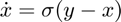
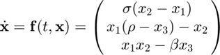
Consider the Lorenz system, with  ,
,  , and
, and  :
:

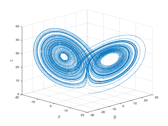
Plot the solution of this system for  in the interval
 ![$[0,100]$](solve_ivp_doc_eq06304400096136047540.png) .
.
First, we can rewrite this system in vector form by letting  ,
,  ,
,  , and
, and  .
.
Defining the system and its initial condition in MATLAB,
% Lorenz parameters
rho = 28;
sigma = 10;
beta = 8/3;

% Lorenz equations in vector form
f = @(t,x) [sigma*(x(2)-x(1));
            x(1)*(rho-x(3))-x(2);
            x(1)*x(2)-beta*x(3)];

% initial condition
x0 = [0;
      1;
      1.05];
Solving the system for in the interval using the classic RK4 method with a time step (i.e. step size) of  ,
,
[t,x] = solve_ivp(f,[0,100],x0,0.001);
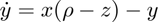
Plotting the solution,
figure;
plot3(x(:,1),x(:,2),x(:,3));
view(45,20);
grid on;
xlabel('$x$','Interpreter','latex','FontSize',18);
ylabel('$y$','Interpreter','latex','FontSize',18);
zlabel('$z$','Interpreter','latex','FontSize',18);
Example #2: Event detection.
Consider the initial value problem
Find the solution  until
until  .
.
First, let's define our ODE ( ) and initial condition in MATLAB.
f = @(t,y) y;
y2 = 3;
Next, let's define the event function,  . Since we want to continue solving until , we want the solver to run while
  ; this forms our condition. Therefore,
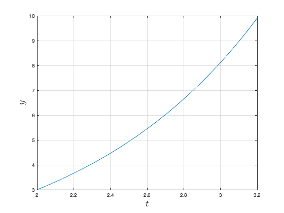
E = @(t,y) y <= 10;
Solving for  using the Euler method with a step size of
  ,
,
[t,y] = solve_ivp(f,{2,E},y2,0.01,'Euler');
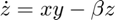
Plotting the solution,
figure;
plot(t,y,'LineWidth',1.5);
grid on;
xlabel('$t$','Interpreter','latex','FontSize',18);
ylabel('$y$','Interpreter','latex','FontSize',18);
Example #3: Backward integration (time detection case).
Consider the same ODE as in Example #2, but we are now given its value at  .
.
Find  . Then, confirm your result by solving the same ODE from
  to , using as the initial condition.
In this case, we know at , and want to find at a previous time . To do this, we need to solve the ODE backwards, from to . First, let's define our ODE () and initial condition in MATLAB.
f = @(t,y) y;
y20 = 50;
Solving for from to using the ABM8 method with a step size of  ,
,
[t,y] = solve_ivp(f,[20,10],y20,0.001,'ABM8');
The solution for corresponding to will be located at the last element of the solution matrix, since is stored in the last element of the time vector. Therefore, is
y10 = y(end)
y10 =

   0.002269996488128
Confirming our result by solving the same ODE but from to and using our result for as the initial condition,
[t,y] = solve_ivp(f,[10,20],y10,0.001,'ABM8');
y20 = y(end)
y20 =

  49.999999999999226
Example #4: Backward integration (event-detection case).
Once again, consider
Find using an IVP solver with a event function (i.e. event-detection).
First, let's define our ODE () and initial condition in MATLAB.
f = @(t,y) y;
y20 = 50;
The event that terminates the solver is when . Therefore, we define the event function as
E = @(t,y) t > 10;
In the time-detection case (Example #3) we input [t0,tf] = [20,10], so the solver knew to integrate backwards in time since t0 > tf. Consequently, internally, the solver made the step size negative. However, for the event-detection case, just given t and E(t,y), the solver won't know to use a negative step size to integrate backwards in time. Therefore, we must manually specify a negative step size. Solving for ,
[t,y] = solve_ivp(f,{20,E},y20,-0.001,'ABM8');
y10 = y(end)
y10 =

   0.002272267619989
Note that this is the same result we obtained earlier in Example #3.